
Comparing Local Residents’ Willingness to Pay (WTP) and Willingness to Volunteer (WTV) for Water Onion (Crinum thaianum) Habitat Conservation


1
Royal Forest Department, 61 Phahonyothin Rd, Lat Yao, Chatuchak, Bangkok 10900, Thailand
2
Department of Forest Sciences and Landscape Architecture, Wonkwang University, 460 Iksan-daero, Iksan 54538, Korea
3
Department of Forest Resources, Yeungnam University, Gyeongsan 38541, Korea
*
Authors to whom correspondence should be addressed.
Forests 2022, 13(5), 706; https://doi.org/10.3390/f13050706
Submission received: 12 March 2022
/
Revised: 28 April 2022
/
Accepted: 28 April 2022
/
Published: 30 April 2022
(This article belongs to the Section Forest Economics, Policy, and Social Science)
Abstract
:In subsistence economies where cash is scarce, non-monetary numeraires can be used instead of cash as utility measures. In this study, we investigate the values of the Thai water onion (Crinum thaianum) (WO), an endangered native wetland plant, for each service enhancement in Thailand, by using willingness to pay (WTP) money and willingness to volunteer (WTV) to measure the value of WO habitat conservation outcomes, including biodiversity, water quality, upstream conditions, and recreational opportunities. This study employs choice experiment (CE) surveys and face-to-face interviews with villagers in the WO areas of Phangnga and Ranong provinces in southern Thailand. The results show that improved upstream conditions are the most important benefit for residents, followed by biodiversity and water quality. Improving upstream conditions, biodiversity, and water quality from low to high would increase estimated annual welfare by USD 89 per person, while local residents would also provide an annual WTV of 80.2 days per person in exchange for considerable improvements in upstream conditions, biodiversity, and water quality. We found that low-income people are more likely to provide labor to improve ecosystem services. Overall, the findings suggest that the labor value, just as the monetary value, can also be used to evaluate the preferences for increased ecosystem services. This study implies that employing volunteer labor as a means of payment for accurate welfare estimations might be a practical alternative, and also allowing respondents to indicate their WTV may lead to an increase in the estimated value of ecosystem services.
1. Introduction
The water onion (Crinum thaianum J. Schulze) (WO) is an endangered native plant occurring only in a few flowing streams in the provinces of Phangnga and Ranong in southern Thailand [1,2]. This plant species plays a significant part in the ecology of a riverine wetland forests. The WO offers food and adequate living areas for native fish and biodiversity. It is a bio-indicator of the wetland forests, growing in clear water [3,4,5,6]. It aids in reducing the speed of water flow, thus stabilizing river soils and ensuring a steady supply of clean water [2]. The WO enhances local livelihoods and economies by providing scenic beauty, especially during the blossom season of October and November, and by serving the recreational sector [7].
Eighty percent of all previous WO communities have unfortunately vanished due to various threats [8]. Overexploitation for commercial uses as aquarium plants and makeup products was formerly thought to be the most serious challenge to WO. Currently, habitat loss and alteration caused by water drainage, especially dredging of river channels to avoid flooding, pose the greatest threat to this species. These activities result in fast-moving water and intensified scour, causing whole WO communities to be uprooted. This has been associated with urban developments and upper catchment degradation, such as land conversion for rubber and oil palm plantations, which have resulted in nitrogen and sediment loading into waterways, resulting in poor water quality and degraded environments for WO [2]. The WO is now classified as “endangered” by the IUCN Red List, and if current trends hold, it could soon be classified as “critically endangered” [9].
Because of intrinsic and non-financial benefits, the importance of species and habitat protection is often taken for granted in decision-making [10,11]. As a result, estimating the social value of plant species and their ecosystem services is important. For example, the government must be able to consider the monetary importance of WO and its wetland ecology while deciding between preserving WO and leasing the loss of its wetlands for flood control, urbanization, or agriculture extension. Benefit–cost analysis is the term for this inquiry. Moreover, the monetary value is important evidence for society and use for biodiversity preservation [12]. Furthermore, public preferences for various qualities of ecosystem services offered by the species and its habitat will aid in the creation of ecological restoration frameworks [13]. It is possible to devise strategies or programs that are more tailored and achieve the highest net gain by understanding which service features in the components are valued by the public [14].
In response, economists have devised a variety of non-market-based methods for estimating or calculating the value that people put on ecological services and presenting those values in monetary terms. There are two types of non-market valuation techniques: revealed preference [15,16] and stated preference [17]. The revealed preference techniques estimate meaning from people’s observed actions, while the stated preference techniques depend on people’s reactions to direct questioning or hypothetical scenarios. Hence, stated preference methods can be used to value both use and non-use values, while revealed preference methods can only be used to value uses, such as recreational facilities and scenic beauty [18,19,20].
According to the Total Economic Valuation (TEV) Framework, the economic value of an ecosystem can be derived from the uses of the services it provides, either consumptive or non-consumptive uses, or even its existence in the absence of use [21]. The task at hand is to determine the non-use values of the advantages offered by species or habitat diversity, as well as to solve the issue of decision-making in the absence of TEV and market prices [22]. The addition of non-use values, such as bequest, altruism, existence, and option values, could boost the advantages of biodiversity protection and tip the balance in favor of saving natural habitats against other economic outcomes. Therefore, the application of stated preference-based approaches has become a major research topic [23]. Contingency valuation (CV) and choice experiment (CE) are the most widely used stated preference methods for capturing non-use value [24]. The CV method can be used to measure a complete change in an area, while the CE method can be used to value multidimensional environmental changes [16]. Likewise, CE can help us to identify one’s preference for each attribute of environment goods and this is meaningful because stakeholders are generally interested in finding out which of the individual attributes contribute to overall changes [14]. As a result, the CE assumes responsibility for determining the most suitable methods for calculating different categories of ecosystem services [25,26,27]. It allows for the calculation of the relative value of various environmental attributes and attribute levels [28,29].
Even though several surveys have been carried out to measure the importance of endangered species, in general, charismatic species are more likely to be conserved, and respondents place a higher value on them or claimed willingness to pay (WTP) [30,31,32,33]. The WTP of marine animals is likely to be higher than that of terrestrial animal species [34]. Although there is clear evidence that the public supports and is willing to pay to conserve charismatic animal species, the literature on the WTP for protecting endangered plant species is noticeably lacking [12]. Besides, the data on the financial benefits of wetland plant species are limited, especially in Thailand, despite the need for the government to prepare and communicate ecological strategies based on precise data.
Additionally, WTP responses are likely to be nil in developing countries where household incomes are very low and local people’s budgets are too tight to give up any portion of their income for biodiversity conservation. As a result, some studies indicate that in subsistence economics where cash is scarce, non-monetary numeraires can be used instead of cash as utility measures [35,36]. However, in the Thai context, we do not have enough information about the use of non-monetary payment vehicles, especially labor contributions or willingness to volunteer (WTV), in ecosystem service valuation.
This study aims to overcome the issue of endangered plant species valuation in low-income communities. In Phangnga and Ranong provinces, we use a choice experiment approach to explore residents’ preferences for four key ecosystem services offered by the WO conservation (i.e., biodiversity, water quality, upstream condition, and recreational opportunity). We assess their willingness to pay money (WTP) and volunteer labor (WTV) in support of WO conservation projects that improve these ecosystem services. We also look at what factors impact residents’ WTP and WTV choices. This study adds to the existence of knowledge in two ways. First, it provides values to different WO conservation outcomes, which are critical pieces of information for creating effective WO population and habitat protection strategies. Second, the study contributes to the non-market valuation literature by employing a volunteer labor as a non-monetary payment mode in choice experiments for welfare estimates in low-income contexts.
2. Materials and Methods
2.1. Choice Experiments for Non-Market Valuation
The CE approach emerged from conjoint analysis, an attribute-based method (ABM) widely used in marketing, transportation, and psychology research [24,37,38], but these days actively applied to environmental economics research [24,39]. People’s preferences for a good’s characteristics are elicited in the initial conjoint study, which involves creating imaginary or hypothetical market conditions. However, some functional issues may arise when using conjoint analysis ranking or rating techniques. Respondents, for example, can find it difficult to rate a large number of options. Consumers are not usually confronted with ranking or rating options. Furthermore, rather than behavioral theory, traditional conjoint analyses are focused on mathematical and methodological concerns [40,41]. The CE, which is a branch of ABMs, differs from traditional conjoint analysis in that participants are asked to select an option from a list of options rather than ranking or scoring them [24]. The CE method’s basic premise is that respondents are decision-makers who are supposed to increase their utility by making a particular option in a given situation [42]. The CE approach tries to replicate an actual demand for a non-market good described by a series of characteristics. In practice, a person first determines the possible choices, considers the characteristics of each choice, then uses the utility maximization decision rule to choose an alternative from a collection of options. As a result, an individual chooses the option with the greatest utility. A selection of attributes and attribute levels distinguish the choices. Since cost is a numerical feature of the good and choice, a marginal rate of substitution between these attributes and money is calculated [24]. This approach will help the researcher determine the welfare transition from the status quo since the status quo is normally included in the option package [43]. It also reflects the price consumers can pay for one of any of the product’s attributes. It is possible to predict the importance people put on improving the qualities of environmental products, or the amount of money they are willing to pay to prevent an adverse feature of the good that they do not value in this manner [24].
Lancaster’s characteristic theory of value [44] and random utility theory are combined to form the CE [45,46]. The total utility obtained from a product or service is the number of individual utilities provided by the characteristics of that good, according to Lancaster’s demand theory [44]. It means that people derive utility or happiness from a good dependent on its properties or characteristics, rather than from the good itself [47]. For example, some people will enjoy a fishing trip even better if it is on a comparatively pristine river with few people, while others may choose to fish on a lake with many people [48].
The random utility model assumes that an individual chooses the choice with the highest utility and that each individual’s utility for option j (Uj) is made up of two components: a measurable proportion (Vj) and a random proportion (εj), or the proportion of utility unknown to the observer. The utility that an individual derives from a particular choice j can be calculated as:
The utility maximization rule says that from a set of possible options, a person will choose the choice that maximizes his utility. In other words, if Uj > Um for all m ≠ j, a person would choose choice j. Assume that an individual chooses choice j, which has the highest utility. After each alternative has been tested, the probability of choosing choice j is proportional to the probability that the utility of choice j is greater than the utility of choice m. Since utilities have an error aspect, the probability that anyone will choose option j can only be expressed as follows:
where C denotes the list of all available choices The conditional logit (CL) model, according to McFadden [49], gives the likelihood of a person choosing choice j if the error fraction in Equation (2) is independent and identically distributed (IID) with an extreme value distribution of form I. The CL model, which says that the inclusion or elimination of other choices has no effect on the relative probabilities of two choices being chosen, is as follows:
A scale parameter λ, which is inversely proportional to the variance of the error term, and a position parameter δ define this distribution. The regular Gumbel distribution of λ = 1 and δ = 0 is usually used in practice [50]. If the measurable proportion (Vj) of utility is linear in the parameters, the individual’s indirect utility function for choice j is typical of the form:
where αi is an alternative status quo, Xk denotes the ecosystem attributes associated with the alternative and a cost attribute expressed in either cash or time. Zs is a vector representing individual characteristics, and αi, βk, and γs are parameters [51,52]. Individual characteristics can be included in the model by interacting them with the alternative status quo. The model incorporates the considered ecosystem attributes through impact codes. According to Hanemann [53], the calculation of increases in wellbeing associated with a decrease in the degree of an attribute is as follows:
where CV is the compensating variation and is the marginal utility of income; Vj0 and Vj1 are the utility before and after the adjustment under consideration. We may use Equation (5) to estimate CV as the welfare estimations of moving from the status quo to the non-status quo (medium and high) levels, where CV is the marginal utility of income; Vj0 and Vj1 are the utility before and after the adjustment under consideration [49]. Equation (5) is simplified when the choice set only includes a single before and after alternative.
Equation (6) shows that the marginal rate of substitution between ecosystem service attributes and cost attributes is simply the ratio of their coefficients for a linear utility function [39]. Therefore, the ratio of the coefficients can be used to describe a marginal WTP (MWTP) value of a shift within a single attribute k:
where βk is the coefficient of the attribute k and µ is the coefficient of the monetary attribute k. The marginal rate of substitution between the cost adjustment and the attribute in question is effectively provided by this partial value formula [40]. Similarly, a marginal WTV (MWTV) value of a transition within a single attribute k can be expressed as a ratio of coefficients, as seen in Equation (8):
where µ is the coefficient of the time attribute and βk is the coefficient of the attribute k. The marginal rate of substitution between cost adjustment and the attribute in question is essentially calculated using this part-worth calculation [40].
2.2. Payment Modes for Non-Monetary Valuation in Developing Countries
According to recent research, the WTP is likely to be zero in countries where household incomes are low and local people’s budgets are too tight to give up any portion of their earnings for environmental protection. However, the payment method chosen may not be appropriate to reflect the preference of people in low-income countries for ecosystem services [54]. Recent stated preference studies in developing countries have used non-monetary payment modes as a utility measure or valuation of various environmental goods and services [54,55,56,57,58,59]. According to Ahlheim et al. [35], non-monetary payment vehicles will reduce the proportion of zero bids. Allowing respondents to express their willingness to provide volunteer labor raises the estimated value of forest ecosystem services, according to Vondolia and Navrud [60]. Depending on the situation, respondents may favor labor donations over monetary donations [61,62,63,64].
For instance, primary forest users (e.g., females, farmers, indigenous community members, etc.) with lower levels of income or education are more likely to be willing to provide labor than monetary contributions [64]. Likewise, half of the Bangladesh respondents reported that they are unable to pay monetary terms, but are willing to contribute in kind for a common level of flood protection [62]. Moreover, rural famers, especially with a greater number of family members, in Nepal were willing to contribute both cash and labor for forest management activities to mitigate damages caused by invasive plant species in a rural area [63].
Other in-kind commodities, such as rice and beehives, have been used in some studies to resolve the cash constraint problem [65,66,67,68]. Brouwer et al. [66], for example, investigated the role of in-kind payment modes in moving from zero cash bids to positive non-monetary bids using a dichotomous option CV of flood control policy in Bangladesh. They discovered that 75 percent of respondents were willing to donate labor, 20 percent were willing to donate harvests, such as rice, and the remaining 5 percent were willing to donate land for the construction of a bank to mitigate flood damage. As a result, the availability of volunteer workers has been seen as a practical scenario for low-income welfare measures [57,69,70,71,72]. Several CV studies have shown that the expected willingness to contribute labor is more likely to exceed the WTP. For example, according to O’Garra [71], willingness to contribute time is three times greater than the willingness to contribute money. According to Lankia et al. [72], respondents’ WTP was higher in terms of labor than income. Furthermore, income has been shown to have a negative impact on willingness to contribute labor.
However, in stated preference surveys, using labor and other non-monetary payment forms as cost contributors poses theoretical challenges [68]. Ahlheim et al. [35], for example, argue that a CV survey based on labor participation conducted in Vietnam does not provide a credible and substantive decision rule for the allocation of funds for public projects because the economic value of the number of labor days reported by individuals is profound to the value of labor, which is condition dependent.
In addition to the CV process, the CE will investigate preferences using non-monetary payment modes. For example, Ando et al. [73] used a CE to assess the benefits of enhancing stormwater management in terms of reported WTP money and willingness to sacrifice time in two major U.S. cities. This study found that people were able to volunteer their time for programs worth 1/3 of the average wage rate, and people benefited from volunteering. Vondolia and Navrud [60] used a CE to evoke preferences among smallholder farmers in developing countries for flood risk mitigation and flood insurance attributes. They discovered that respondents’ attitudes toward money, labor, and harvest payment modes were all similar. Non-monetary payment vehicles’ relative scale parameters, on the other hand, were found to be lower than monetary payment vehicles’ relative scales. Rai and Scarborough [67] assessed the implied prices for each payment mode by adjusting for a means of payment using dual cost attributes, that is, monetary and labor attributes combined in CE. The dual cost attribute can make interpreting results difficult. Then, they used a two-stage CE to enable respondents in the Chitwan National Park buffer zone in Nepal to express their willingness to contribute in the form of labor if they did not want to pay in cash. Male migrants with higher education and households with higher non-farm income were more likely to perform the money option mission, according to the binary logistic model’s findings. Respondents from the buffer zone or with a larger family, on the other hand, were more likely to prefer employment as a source of income [68].
Our study, thus, focuses on how non-monetary payment vehicles reflect the preference of people for ecosystem services better than monetary payment vehicles. Furthermore, we investigate the different preference of people by the type of ecosystem services, and also socioeconomic impacts on the amount of WTP for ecosystem services.
2.3. Description of the Water Onion and Its Habitats
The water onion, water lily, Thai water onion, onion vine, and yellowish leaves lily are all common names for Crinum thaianum J. Schulze, an aquatic plant in the Amaryllidaceae family [1]. This species reproduces primarily by vegetative means, with a mother bulb producing several smaller bulbs, which are visible as clusters of bulbs emerging in the stream (see Figure 1).
The WO is an endemic endangered wetland plant found only on Thailand’s upper southwest coast, in the provinces of Ranong and Phangnga, stretching 110 square kilometers from Ranong’s Kapoe and Suksamran districts to Phangnga’s Khura Buri and Ta Kua Pa districts [1] (see Figure 2). This wetland plant survives in a unique environment, particularly in canals with clear water and sunlight passing through to the canal bed [74]. According to a survey in 2008, there are ten canals where WO can be found. These canals ran from Kapoe district, Ranong province, south to Ta Kua Pa district, Phangnga province, covering a total area of approximately 17,168 square meters. However, between 2010 and 2011, the distribution of WO decreased to 5,456 square meters. In 2013, the Thailand Institute of Scientific and Technological Research (TISTR) performed a survey and discovered that the WO is no longer present in certain locations. The study also discovered that the number of WO exit sites has been steadily decreasing. Since 2008, the area of WO distribution in some canals has declined by more than 50 percent. For example, the WO area in the Naka canal of Ranong province’s Suksamran district decreased from 8832 square meters in 2008 to only 208 square meters in 2013. Similarly, the Bang Pong canal in the Khura Buri district of Phangnga province had 3760 square meters in 2010, but just 278.4 square meters in 2013. This may imply the WO is critically endangered. Finally, the TISTR completed a survey of the area where the WO was found in 2016, discovering a total of 18 canals with a population of 12,824 square meters, as well as a small increase in the presence of WO [74].
Since this plant species has a limited range of habitat, the extinction of a single organism could result in the extinction of the entire species if proper management practices are not implemented [75]. As a result, the WO-rich areas of Phangnga province’s Khura Buri district and Ranong province’s Suksamran and Kapoe districts were chosen as study areas.
2.4. Choice Experiment Design
In this study, we set two research hypotheses:
Hypothesis 1.
In low-income countries, non-monetary payment vehicles reflect the preference of people for ecosystem services better than monetary payment vehicles. (Null hypothesis: there is no difference between non-monetary payment vehicles and monetary payment vehicle in terms of the amount of payment for ecosystem services in low-income countries).
Hypothesis 2.
People have a different preference by the type of ecosystem services. (Null hypothesis: there is no difference in terms of preferences by the type of ecosystem services).
Hypothesis 3.
Socioeconomic status has an impact on the amount of WTP for ecosystem services. (Null hypothesis: there is no difference in terms of the amount of WTP by socioeconomic status).
Thus, we used CE surveys and interviewed people in the research area to evoke their interests, WTP, and WTV for enhancing ecosystem services gained from the conservation of WO and its wetland ecosystem. In order to ensure the validity and reliability of the results estimate through CE research, the study was carefully designed considering commonly occurring biases [76], such as information sequencing effects. Kjaer et al. [77] omitted attributes. The current status of ecosystem services is believed to be low (status quo). Two new conservation proposals were given to respondents. These plans will ensure that the ecosystem services that are considered are improved. A monetary donation or labor contribution was used as a WTP or WTV measure attribute, respectively. However, to calculate a given marginal WTV, we only used samples from Ranong province in which respondents performed CE tasks in both monetary and labor terms.
The selection of attributes and their levels is the first step in designing a preference experiment. Based on fieldwork, literature analysis, and interviews with local citizens and ecologists who are specialists in wetland and WO management, the characteristics correlated with the outcomes resulting from WO conservation programs were established. Biodiversity, water quality, upstream condition, and recreational opportunity were chosen as the four ecosystem service attributes as a consequence. The selection of attributes and their levels is the first step in designing a preference experiment (Table 1, Table 2 and Table 3) and this was conducted based on suggestions from the previous studies. Specifically, Schultz et al. [78] reported that when we set up a scenario, baseline and change should be presented in precise, measurable, and interpretable terms. According to Johnston et al. [79], inaccurate technical terms, such as “high,” “medium,” or “low” by respondents, should be clearly defined and should not be used if they do not understand it. Moreover, the presented outcome should allow respondents to clearly identify objectives and outcomes [80]. Furthermore, the characteristics correlated with the outcomes resulting from WO conservation programs were established based on fieldwork, literature analysis, and interviews with local citizens and ecologists who are specialists in wetland and WO management. As a result, biodiversity, water quality, upstream condition, and recreational opportunity were chosen as the four ecosystem service attributes. As indicated in Table 1, these four characteristics are divided into three levels (low, medium, and high). Biodiversity was described as the abundance and variety of WOs, fish, insects, animals, and other aquatic species. It denotes a non-use value. The low level indicates that the wetland contains a small number of water onions, fish, insects, animals, and other aquatic species. At the medium level, the abundance and variety of water onions, fish, insects, animals, and other aquatic species have increased by 25%. The high level refers to a scenario in which the abundance and variety of aquatic species, such as water onions, fish, insects, animals, and other aquatic species, have grown by 50%. The second attribute, indirect value, was chosen as a proxy for water quality. When performance is low, odors and algae become visible. The medium level suggests somewhat muddy water with visible algae but no smell. The high water quality is crystal clear and odorless. The third feature considered was the upstream condition, which reflects the density of upstream and riverside plants, as well as the degree of bank erosion. Low: there is a lack of upstream and bank vegetation, and erosion is common at this level. There is a moderate level of upstream and bank vegetation, as well as a moderate risk of erosion, at the medium level. The recreational opportunity reflects a non-consumptive use-value. Only visual amenity is available at the low level. Secondary contact recreation, such as fishing, rafting, and boating, is possible at the medium level. At the highest level, all types of recreation are available, as well as the development of tourism infrastructure.
According to Rai and Scarborough [64], using two cost-attributes, monetary and labor, as attributes in the CE will enhance the sophistication of the results review. In this study, we used the cost attribute in monetary or labor donations to help WO conservation projects that strengthen wetland ecosystem services. The monetary contribution is a one-year grant to the WO conservation project. Respondents were asked open-ended questions during the pilot test period to express their desires for monetary donation and labor commitment. Thus, the survey’s monetary and labor payment amounts were chosen from the top-four ranking frequencies of respondents in the pilot test of 50 individuals conducted in Phangnga province. There were THB 50 (USD 1.5) to THB 100 (USD 3), THB 200 (USD 6), and THB 400 (USD 12). The labor allocation is the number of days that respondents will spend taking steps to strengthen ecosystem services. We demonstrate that events must be available for people of all abilities, and the province would keep track of the work. Labor days are divided into four categories: 2, 4, 6, and 12 each year. Table 1 lists this attribute and their levels.
The next step is to create CE tasks from the selected attributes. We first create the CE task in monetary terms by using a typical preference modeling experimental design with non-status-quo choices in choice questions being assigned attributes and levels according to an orthogonal factorial main effects design [82]. However, the number of potential configurations or possibilities based on the chosen characteristics is enormous, and it is difficult to include all of them in the survey. To create a more tractable CE survey, we used the fractional factorial and orthogonal styles in SPSS. As a result, forty possibilities representing the first alternatives in of choice set (Plan A) were created to cover the spectrum of uncertainty between all possible combinations [83].
Then, as an extension of the orthogonal strategy, the cyclical design was used to derive the second alternative (Plan B) from a particular Plan A. As a result, each choice set includes two different plans (Plans A and B). Each choice set also included the status quo, which resulted in a low condition in all ecological resources due to the lack of conservation projects. The forty choice sets were then divided into ten blocks, each with four choice sets. In monetary terms, the CE task is divided into ten versions.
We planned the CE task in labor contributions after we developed the CE task in monetary terms. This mission has a labor contribution as an expense attribute instead of a cash donation. The labor contribution is the number of days a respondent will spend on things such as harvesting seeds, transplanting, replanting, upstream forest preservation, erosion prevention, and promoting youth education about wetlands and WO protection, enhancement, and conservation. The sum of money in THB (50, 100, 200, and 400) was replaced with the number of labor days (2, 4, 6, and 12), respectively. Then, we reordered the forty choice sets into ten blocks (1B–10B). Table 2 and Table 3 show an example of a choice set for the CE task in monetary terms and the CE task in labor contributions, respectively.
2.5. Questionnaire Design
The key questionnaire used in this analysis is divided into three parts. The first section of the questionnaire covers socioeconomic characteristics, such as gender, marital status, age, education, profession, income, and household size. The second section contains questions about respondents’ perceptions of the advantages of WO and risks to the WO and its wetland habitat, conservation interactions of WO, and perceptions of conservation initiatives for this species. The final section is about the choice experiment task in monetary terms. In addition, to evoke the WTP of respondents in Ranong province, we added the following CE task in volunteer labor terms and its relevant queries.
2.6. Field Trial/Survey
A 30-person pilot test was conducted prior to prescribing the final sample to ensure that the characteristics selected, and the choice experiment tasks were acceptable. According to Johnson and Orme [84], the minimum sample size requirements for the CE depend on the number of choice sets (t), the number of analysis cells (a), thus the minimum sample size (N) is calculated using the following equation. When considering main effects, c is equal to the largest number of levels of any attributes:
We then performed two face-to-face interview surveys in June and December 2019. The survey participants were selected at random from the WO-rich areas of Phangnga and Ranong provinces. The first survey using the CE task in monetary terms (questionnaire versions 1A–10A) was conducted in June 2019 in Khura Buri district, Phangnga province. As a result, 101 people were assigned to one of ten different monetary-based questionnaire versions at random. Participants were asked about their socioeconomic status, their perceptions of the benefits of WO, WO risks, and future management strategies, as well as their experiences with voluntary WO conservation. Then, in the CE section, the interviewer presented respondents with background information about WO and its wetland ecosystem using cards and pictures. Typically, this stage consists of the CE task in monetary terms. All respondents were first asked to complete four choice sets, each of which allowed them to choose between two possible WO conservation outcome scenarios and the status quo.
The second survey was performed in Ranong province’s Suksamran and Kapoe districts in December 2019. The CE task in monetary terms, as well as the CE task in labor terms, are all included in this survey. In the CE section, 166 respondents were first assigned to one of ten versions (1A–10A) of the CE task in monetary terms, which consisted of four choice sets. After that, they were asked to replicate the process for the CE task in labor terms (1B–10B), which also had four different sets of questions. For instance, a respondent who was initially asked to complete the 1A form was also asked to complete the 1B version. As a result, respondents were given eight different choice sets to choose from.
Finally, all 267 respondents were asked to complete the CE task in monetary terms, with 166 in Ranong province being asked to complete the CE task in volunteer labor terms as well. As a result, we gathered data from two treatments: monetary (267 respondents) and labor (166 respondents).
2.7. Model and Welfare Estimation
In the CE tasks listed above, each respondent was asked to select one of two conservation outcomes or the status quo choice to determine whether or not to support the WO conservation project. Every respondent was given four separate choice sets to answer in each CE task. Therefore, each respondent gave one answer for each choice set, which was registered alongside the alternative levels for the two hypothetical conservation plans and the status quo option. There are 4 × 3 = 12 data points for each respondent.
All ecosystem attributes are coded using impact codes (“1”, “−1”, and “0”) when coding the attribute levels. When the base preference is presented, the status quo option’s coding attribute levels are normally treated the same way as the other preference alternatives [82]. One level is included as the status quo for the four considered ecosystem service attributes of three levels, and two results code variables are generated for the other two levels. For example, we applied a low level as the status quo level and two variables (medium and high level of biodiversity improvement) to the data set while coding the biodiversity parameter. As a consequence, the present condition has been assigned the code “−1.” When the moderate level was included in the alternative, it was coded as “1” and the high level was coded as “0.” On the other hand, the high was coded as “1” and the moderate was coded as “0” where the high level was the included level of the option [83]. Then, we used LIMDEP 9.0 tools to approximate CL models for MWTP and MWTV values.
3. Results
3.1. Respondents’ Socioeconomic Characteristics
Table 4 shows the primary socioeconomic status of the respondents. A total of 267 people responded to the money treatment, and 166 people responded to the voluntary labor treatment. The participants in the money treatment were largely male (57 percent) and ranged in age from middle-aged to elderly, with an average age of 46. A 35–49-year-old group accounted for 44 percent, while the 50–64-year-old group accounted for 33 percent. Most respondents were married (72 percent). Below high school was the most common educational standard (39 percent), followed by high school (36 percent) and undergraduate (22 percent). Farmers (36 percent) were the most common occupation among respondents, followed by civil servants (33 percent), self-employed (15 percent), employees (12 percent), and others (5 percent). The average monthly income of the respondents was THB 13,232 (USD 382), with an average family size of 3.8 individuals. Most responders were from Ranong province, with 43% from Kapoe district and 19% from Suksamran, and the remaining 30% from Phangnga province’s Khura Buri district.
The socioeconomic characteristics of the labor treatment sample are similar to those of the money treatment. The majority of those who responded were men (61 percent). Participants ranged in age from 18 to 64, with an average of 46. Eighty-one percent of respondents were married. The most common educational standard was high school (42 percent), followed by below high school (40 percent) and undergraduate (15 percent), respectively. Farmers were likewise the most common occupation in the volunteer labor therapy, followed by civil servants. With a medium-sized family of 3.9 individuals, the respondents’ average monthly income was THB 12,632 (USD 379). All of the respondents were from Ranong province, with 70% being from Kapoe and 30% coming from Suksamran.
3.2. Respondents’ Attitudinal Characteristics
Table 5 summarizes respondents’ perspectives on WO benefits and risks, as well as their experiences with WO conservation. For the money treatment, most of the respondents (87 percent) had known about the benefits of WOs. They believe that this plant species provides recreation values, water purification, and income for the local community. Furthermore, the majority of respondents believe that river dredging and expansion for flood control is the greatest danger to the WO its wetland habitat, followed by commercial exploitation as aquarium plants. Environmental organizations made up 49 percent of the overall. The majority of respondents (67 percent) said they had taken part in WO conservation programs, with around 52 percent saying they had taken part through WO breeding and planting. Almost all of the respondents (89 percent) said they would be willing to volunteer to assist in WO conservation efforts. About 80% of respondents agree that WO conservation can be accomplished by voluntary engagement. The volunteer labor treatment yielded similar findings in terms of respondents’ perceptions toward WO.
3.3. CL Model Results
After data collection, the commonly chosen neither alternative responses were classified and omitted from the full sample. Thus, by excluding these answers, 242 usable samples (968 observations) for WTP estimation and 148 usable samples (592 observations) for WTV estimation can be obtained. Data from the CE task in monetary terms (money treatment) and the CE task in labor contribution (labor treatment) are included in the findings. The CL models were calculated using LIMDEP 9.0 software as respondents chose one of the particular choices (Plan A or Plan B) or neither alternative.
Table 6 shows the coefficient estimates for the CL specifications using the money treatment with two models: no socioeconomic variables (Model 1a) and socioeconomic variables (Model 1b). The marginal utility of the four attributes, biodiversity, water quality, upstream condition, and recreational opportunity, is shown in this table at different levels. The regression coefficients can be interpreted as marginal utility values, which represent how individuals’ utility increases or decreases when the attribute level changes [84]. The estimated coefficients obtained from the money treatment in both models (1a,b) show a negative and significant coefficient exists for the money cost attribute. The magnitudes of the service attribute coefficients are all significant and on the predicted sign, with the exception of the recreational opportunity coefficient. The upstream condition and water quality coefficients are significant and positive at the high level. For both medium and high biodiversity, the coefficients are positive and significant. Hence, residents value a high degree of improvement in the upstream condition and water quality, as well as a medium and high degree of increase in biodiversity, whereas residents prefer the current status of recreation attribute. The coefficient of respondents’ age was found to be positive and significant among the socioeconomic factors. Thus, the elderly were more willing to pay money to improve ecosystem services offered by WO conservation.
Table 7 shows the coefficient estimates for the CL specifications from the money treatment of the WO case using two models: no socioeconomic variables (Model 2a) and with socioeconomic variables (Model 2b). This table demonstrates that the labor cost attribute has a negative and significant coefficient. The results are consistent with the previous models in that the coefficient for payment is significant and negative, while all other characteristics are positive and significant excluding recreational opportunity. These results show that a medium to a high degree of change in upstream conditions, as well as a high degree of improvement in biodiversity and water quality, were expected to be vital to respondents. It also implies that respondents are satisfied with the present state of the leisure attribute, which is purely visual amenity. Furthermore, those with lower incomes were more likely to provide labor to improve these ecosystem services among the socioeconomic factors.
3.4. Estimation of Willingness to Pay and Willingness to Volunteer
Table 8 shows calculations of the MWTP and MWTV for changes in the three attributes, namely erosion prevention, biodiversity, and water quality. We used the coefficients on the significant three services and the money payment attribute from Model 1a to calculate the CV for upgrading each service from the status quo to higher levels. As a result, the CV for improving upstream conditions from low to high is 744−(−744), THB 1488 (USD 45) per person per year. The CV for increasing biodiversity from low to high is 428−(−564), THB 992 (USD 30) per person per year, and the CV for enhancing water quality is 235−(−235), THB 470 (USD 14) per person per year. As a result, increasing average welfare by THB 2950 (USD 89) per year by enhancing upstream conditions, biodiversity, and water quality from low to high.
Similarly, we estimated the CV for enhancing all major ecosystem resources using the approximate coefficients from the labor treatment (Model 2a). From the status quo (low) to the high level, upstream conditions take 15.1−(−24.9), 40 days per person per year, biodiversity takes 10.2−(−10.2), 20.4 days per person per year, and water quality takes 9.9−(−9.9), 19.8 days per person per year. Hence, respondents have a WTV of 80.2 days per year for a high improvement in upstream conditions, biodiversity, and water quality to a high level.
4. Discussion
A number of discussion points can be derived from this study. Initially, residents in WO areas of Phangnga and Ranong provinces value upstream conditions first, followed by biodiversity and water quality, and are unlikely to support increased recreational opportunities. It can be inferred that among the ecosystem services examined in this study, the most need of residents is an improvement in upstream conditions. Residents want to see a significant increase in upstream quality. Since the residents reported that they were concerned about river erosion, dredging of the river was identified as the greatest threat to WO. Moreover, although there is a small difference in Model 2 using the labor cost attribute, biodiversity, which is a non-use value, is more important than water quality as an indirect benefit. Residents, on the other hand, were not in favor of expanding recreational opportunities. This means that the current state of recreational opportunities, which is purely visual, is satisfactory to locals.
In the late 2010s, other studies on trade-offs and synergies between detailed properties of ecosystem services have been conducted [85,86,87]. Although still limited, there are studies [88,89] that provide evidence for the potential trade-off between erosion protection and flood protection properties covered in our study. In the meantime, since the definition and classification of ESs must be made during specific decision-making processes differently depending on the target area or situation due to their diversity and complexity [90]. It is also true that the findings from other studies cannot be directly applied to our findings. Instead, our findings, together with the findings from Galicia and Zarco-Arista [88] and Turner et al. [89], may help the government and local authorities in making policy decisions to avoid floods. Perhaps, the government may start considering employing the benefit−costs analysis to compare the standard costs for flood prevention and the impact on WO habitat conservation.
Furthermore, the CE situations can be used to determine the WTP and WTV values in a specific way. For example, as shown in Table 6, improving upstream condition, biodiversity, and water quality, to high-level yields average welfare of USD 89 per year. According to the results of a CE report conducted by Ando et al. [73], people value improving aquatic health from fair to outstanding, and water quality from boatable to swimmable in lakes and rivers as much as USD 294 per household per year in Chicago, and USD 277 per household in Portland. Thus, our average value is significantly smaller than that of Ando et al. [73]. This backs up the statement that respondents in developed countries are likely to pay more money than respondents in developing countries [36]. However, it is consistent with the results of Seenprachawong [83], who conducted an earlier CE analysis in the adjacent region of Phangnga Bay and found a WTP of USD 71 per year for the improvement of the Phangnga Bay ecosystem. Furthermore, we discovered that the WTP for restoring the endangered wetland species (Nymphoides peltata) in Japan, which is around USD 59, is lower than the mean WTP for restoring the WO habitat [91].
In comparison, Phangnga and Ranong residents’ approximate WTP value for conserving WO is two times higher than Bangkok residents’ WTP for restoring the BKGA (USD 42 per person per year). One reason for this is that people are likely to support the conservation of endangered species [8]. Since, residents in Phangnga and Ranong have become involved in WO conservation efforts, making them more aware of the value of protecting this endemic species and its wetland habitat [8].
We also discovered that the most common attribute combination resulting from the labor treatment, which was similar to the money treatment, had an average WTV of 80.2 days per year. Therefore, respondents would be willing to volunteer up to two days per week to help with WO conservation. Because no preference research has been conducted in Thailand, we cannot compare WTV estimates with those from the previous study in the country. In contrast, Shandas [92] discovered that Portland residents would be prepared to volunteer a few hours per month to help reduce stormwater pollution and improve watershed health. Our estimated WTV is also higher than the findings of Ando et al. [73], who found that respondents will be willing to volunteer 50 h a year to increase water quality from boatable to swimmable and conserve aquatic habitat from fair to excellent. Furthermore, our estimated WTV is ten times higher than those calculated by Rai and Scarborough [64], which found that the estimated labor contribution for forest ecosystem services in Nepal was 9.38 days/year. Besides, the WTV of residents for the firebreak establishment and maintenance program in Vietnam was 5 days per year according to the CV data of Hung et al. [67]. In comparison to these previous surveys, our findings show higher WTV values. This might be because residents have a strong desire to participate and are familiar with WO conservation and volunteerism. According to Athihirunwong et al. [8], 57 percent of survey respondents had previous experience with WO conservation, and they observed that youth conservation motivations in Kopoe district, Ranong province, promote actual conservation participation. Furthermore, we observed that 78 percent of labor treatment responders had participated in WO conservation. Therefore, our WTV estimate may be somewhat large.
The results from the money treatment are similar to those of the labor treatment, with a few exceptions. In the money treatment, people benefited from increased biodiversity at a medium or high level, while in the labor treatment, people benefited from improved upstream conditions at a medium or high level. However, the overall data show that preferences for improved ecosystem services from the money and labor treatments were not evaluated differently. The advantage of using the latter model is demonstrated by an increase in the log-likelihood function. This study suggests that using volunteer labor as a payment method for obtaining accurate welfare estimates might be a viable option.
We explored the impact of socioeconomic variables on their WTP and WTV decisions in this analysis. According to our findings, the age of respondents had a positive effect on the WTP for increasing ecosystem services supplied by WO conservation. This may be due to a long period relation with WO that elderly people received [87]. While income is a key factor affecting WTV decisions, the negative effect of income on WTV found in this study may be because people with high income have higher opportunity cost of time. This finding supports the conclusion of Lankia et al. [72] that income has a negative impact on willingness to contribute labor. Although we could not conduct the same surveys in the study areas of Phangnga and Ranong provinces due to the budget and time limit of our study, in Table 2 and Figure 2, results show that the impact of socio-economic factors on WTP and WTV are robust across models in Table 4 and Table 5. Those tables show that our statistical models are robust and also show the consistent results with different model settings.
Ando et al. [73], who used a CE to evaluate the outcomes of stormwater management improvement in terms of reported WTP money and willingness to sacrifice time in two large U.S. cities, found that people were willing to contribute their time for services worth 1/3 of the average wage rate and that people benefited from volunteering. Moreover, the opportunity cost of labor provided by Rai and Scarborough [63] is estimated to be USD 2.33 per day. As a result, we modified this result by converting the approximate WTV of 80.2 days into a dollar value. In 2019, the average wage rate in Ranong province was USD 10 per day, thus, the average value of volunteer labor was worth USD 3 per day. Consequently, the annual cost for 80.2 days was calculated to be USD 240.6 per person. Our results show that WO is highly regarded in the community. Therefore, our findings support the statement that allowing respondents to express their willingness to contribute labor increases the estimated value of forest ecosystem services in developing countries [64].
This study contributes to valuation literature in two respects. First, it improves understanding of the importance of multiple ecosystem services provided by Thailand’s basic life-support systems, the wetlands, and can play an important role in encouraging greater efforts to protect them. We proposed that improving all WO wetland ecosystem services, excluding the recreation service, could improve residents’ utility. This study provides the economic value of WO and its wetland habitats to policymakers so they can determine it is worthwhile to invest in its conservation. Second, the non-payment vehicle is combined with CE valuation processes. The CE was used for the first time in this study to assess people’s preferences and WTV in the context of Thai rural wetlands. It is particularly important because Thailand is a developing country with sufficient volunteer labor for environmental protection efforts. Since Thailand has little experience conducting CE surveys using non-monetary payment vehicles, the applicability and deeper meanings of the estimated value must be considered.
However, while we used a random sampling methodology to prevent statistical bias, we used a small number of survey samples in this research, which may contribute to coverage error in the statistical analysis. A sufficient number of samples is needed to resolve these statistical issues. Future research may compare the difference in mean WTP and WTV between large and small samples to account for this coverage error.
Furthermore, the model used in the two case studies imposes a constraint. Discrete choice models are common because they have an easily interpretable closed-form choice probability and a globally concave likelihood function [88]. The CL model used in this study assumes that respondents are homogeneous and that each error term is distributed independently and identically, which means that the chances of outcomes are unaffected by the availability of other outcomes [88,89]. However, the CL model can only account for respondent heterogeneity in a rather simplified way. Via interaction with the constant words or main design attributes, sources of observed heterogeneity (i.e., socioeconomic, attitudinal, and demographic variables) were integrated into the CL model. Consequently, despite giving respondents enough time to understand the option sets, this model is limited in its ability to answer the impact of repeated choices from the same respondents. Future studies can extend the model by allowing random parameters, particularly to accommodate the heterogeneity of unobserved preferences, due to advancements in statistical programs.
5. Conclusions
In this study, we investigated the preferences, WTP and WTV of rural residents for enhancing ecological services provided by the WO’s wetland ecosystem in southern provinces of Thailand. We used the CE process to explore people’s interests in terms of money and voluntary donations for the WO conservation program. For the calculation, we used both monetary and non-monetary payment modes and discovered that respondents would be willing to pay THB 2950 (USD 89) and work 80 days per year in exchange for a significant increase in upstream condition, biodiversity, and water quality. It can be concluded that the respondents considered improving upstream condition to be the most important ecosystem service provided by the WO, followed by biodiversity enhancement, and improved water quality, but that an increase in recreational opportunities was not relevant. We also discovered that the labor contribution was assessed in the same way as a monetary payment vehicle.
We offer policymakers information on the economic value of WO and its wetland habitat so they may decide if it is worth investing in its conservation. Except for the recreational service, we proposed that restoring all WO wetland ecosystem services might increase inhabitants’ utility. Because enhancing the condition of upstream forests is the most important ecosystem function, followed by increasing biodiversity and improving water quality, we firstly recommend the government increase its efforts to promote upstream forest management and erosion control. The appropriate authorities could take steps to strengthen incentives for private landowners, particularly rubber and oil palm producers, to safeguard WO, such as promoting agroforestry. For example, the government could establish a market where the purchase price of agroforest products is guaranteed. Payment for Ecosystem Services (PES) might be used to allow communities and inhabitants to pay for advantages in exchange for non-use values from WO. Second, channel dredging should be avoided to reduce sediment erosion, preserve wetlands and ecological health, and improve water quality. Monocultures, such as those involving chemicals, should be avoided. Local engagement and volunteerism, in particular, can assist in WO conservation. Finally, because residents are opposed to increasing recreational opportunities, tourism should have a fixed zone to conserve genetic resources. Rather than relying on tourism infrastructure, communities should concentrate on ecotourism and environmental education, which would increase public knowledge and participation in conservation WO.
Author Contributions
A.P. designed the questionnaire, conducted the survey, analyzed the data, and wrote the manuscript; Y.L. supervised, edited the manuscript, and approved the final version; J.-H.J. edited the manuscript and approved the final version. All authors have read and agreed to the published version of the manuscript.
Funding
We acknowledge National Research Foundation of Korea(NRF) funded by the Ministry of Education for funding to support this study(NRF-2021R1F1A1046935 and NRF-2021R1F1A1046935).
Data Availability Statement
Not Applicable.
Conflicts of Interest
The authors declare no conflict of interest.
References
- Schulze, J. Crinum thaianum J. Schulze, a new aquatic species from Southeast Asia. Plant Life 1972, 27, 33–42. [Google Scholar]
- Lansdown, R.V. The Conservation of Aquatic and Wetland Plants in the Indo-Burma Region. In The Status and Distribution of Freshwater Biodiversity in Indo-Burma; Allen, D.J., Smith, K.G., Darwall, W.R.T., Eds.; IUCN: Cambridge, UK; Gland, Switzerland, 2012; pp. 117–133. [Google Scholar]
- Shepard, J.P. Effects of Forest Management on Surface Water Quality in Wetland Forests. Wetlands 1994, 14, 18–26. [Google Scholar] [CrossRef]
- Trettin, C.C.; Jurgensen, M.F. Carbon cycling in wetland forest soils. In The Potential of US Forest Soils to Sequester Carbon and Mitigate the Greenhouse Effect; CRC Press: Boca Raton, FL, USA, 2002; pp. 311–331. [Google Scholar] [CrossRef]
- Kahn, F.; Mejia, K. Palm Communities in Wetland Forest Ecosystems of Peruvian Amazonia. For. Ecol. Manag. 1990, 33, 169–179. [Google Scholar] [CrossRef]
- Prieditis, N. Status of Wetland Forests and their Structural Richness in Latvia. Environ. Conserv. 1999, 26, 332–346. [Google Scholar] [CrossRef]
- Treerutkuarkul, A. Conserving Habitats for Globally Important Flora and Fauna in Production Landscapes Project Result Report; IUCN Thailand Programme: Bangkok, Thailand, 2020. [Google Scholar]
- Athihirunwong, N.; Janekarnkij, P.; Sanglestsawai, S. Understanding Youth Motivation for Water Onion (Crinum Thaianum J. Schulze) Conservation in Thailand. Kasetsart J. Soc. Sci. 2018, 39, 42–50. [Google Scholar] [CrossRef]
- IUCN Species Survival Commission. IUCN Red List Categories and Criteria: Version 3.1; IUCN Species Survival Commission: Gland, Switzerland, 2001. [Google Scholar]
- Costanza, R.; d’Arge, R.; De Groot, R.; Farber, S.; Grasso, M.; Hannon, B.; Limburg, K.; Naeem, S.; O’neill, R.V.; Paruelo, J. The Value of the World’s Ecosystem Services and Natural Capital. Nature 1997, 387, 253–260. [Google Scholar] [CrossRef]
- Bingham, G.; Bishop, R.; Brody, M.; Bromley, D.; Clark, E.T.; Cooper, W.; Costanza, R.; Hale, T.; Hayden, G.; Kellert, S. Issues in Ecosystem Valuation: Improving Information for Decision Making. Ecol. Econ. 1995, 14, 73–90. [Google Scholar] [CrossRef]
- Pandit, R.; Subroy, V.; Garnett, S.T.; Zander, K.K.; Pannell, D. A Review of Non-Market Valuation Studies of Threatened Species and Ecological Communities. Report to the National Environmental Science Programme, Department of the Environment, Canberra, Australia. 2015. Available online: https://www.nespthreatenedspecies.edu.au/publications-and-tools/a-review-of-non-market-valuation-studies-of-threatened-species-and-ecological-communities (accessed on 19 December 2017).
- Christie, M.; Warren, J.; Hanley, N.; Murphy, K.; Wright, R.; Hyde, T.; Lyons, N. Developing Measures for Valuing Changes in Biodiversity: Final Report; Report to DEFFA; DEFFA: London, UK, 2004. [Google Scholar]
- Hanley, N.; MacMillan, D.; Wright, R.E.; Bullock, C.; Simpson, I.; Parsisson, D.; Crabtree, B. Contingent Valuation Versus Choice Experiments: Estimating the Benefits of Environmentally Sensitive Areas in Scotland. J. Agric. Econ. 1998, 49, 122–128. [Google Scholar] [CrossRef] [Green Version]
- Malpezzi, S. Hedonic Pricing Models: A Selective and Applied Review. Hous. Econ. Public Policy 2003, 1, 67–89. [Google Scholar] [CrossRef]
- Bockstael, N.E.; McConnell, K.E. Environmental and Resource Valuation with Revealed Preferences: A Theoretical Guide to Empirical Models; Springer Science & Business Media: Berlin, Germany, 2007. [Google Scholar] [CrossRef]
- Johnston, R.J.; Boyle, K.J.; Adamowicz, W.; Bennett, J.; Brouwer, R.; Cameron, T.A.; Hanemann, W.M.; Hanley, N.; Ryan, M.; Scarpa, R. Contemporary Guidance for Stated Preference Studies. J. Assoc. Environ. Resour. Econ. 2017, 4, 319–405. [Google Scholar] [CrossRef] [Green Version]
- Pearce, D.; Atkinson, G.; Mourato, S. Cost-Benefit Analysis and the Environment: Recent Developments; Organisation for Economic Co-operation and Development: Paris, France, 2006. [Google Scholar]
- Hanley, N.; Spash, C.L. Cost-Benefit Analysis and the Environment; Edward Elgar Publishing Limited: Hants, UK, 1993. [Google Scholar]
- Tunstall, S.M.; Coker, A. Survey-based valuation methods. In Valuing the Environment: Economic Approaches to Environmental Evaluation; Coker, A., Richards, C., Eds.; John Wiley & Sons Ltd: West Sussex, UK, 1996; pp. 104–126. [Google Scholar]
- Pascual, U.; Muradian, R.; Brander, L.; Lopez, B.M. The Economics of Valuation Ecosystem Services and Biodiversity. Econ. Ecosyst. Biodivers. Ecol. Econ. Found. 2010, 183–256. [Google Scholar] [CrossRef]
- Heal, G.M.; Barbier, E.B.; Boyle, K.J.; Covich, A.P.; Gloss, S.P.; Hershner, C.H.; Hoehn, J.P.; Pringle, C.M.; Polasky, S.; Segerson, K. Valuing Ecosystem Services: Toward Better Environmental Decision-Making; National Academies Press: Washington, DC, USA, 2005. [Google Scholar]
- Tisdell, C.A. Economics of Environmental Conservation; Edward Elgar Publishing: Cheltenham, UK, 2005. [Google Scholar]
- Adamowicz, W.; Louviere, J.; Williams, M. Combining Revealed and Stated Preference Methods for Valuing Environmental Amenities. J. Environ. Econ. Manag. 1994, 26, 271–292. [Google Scholar] [CrossRef]
- Shoyama, K.; Managi, S.; Yamagata, Y. Public Preferences for Biodiversity Conservation and Climate-Change Mitigation: A Choice Experiment using Ecosystem Services Indicators. Land Use Policy 2013, 34, 282–293. [Google Scholar] [CrossRef]
- Chaikaew, P.; Hodges, A.W.; Grunwald, S. Estimating the Value of Ecosystem Services in a Mixed-use Watershed: A Choice Experiment Approach. Ecosyst. Serv. 2017, 23, 228–237. [Google Scholar] [CrossRef] [Green Version]
- Jang-Hwan, J.; So-Hee, P.; JaChoon, K.; Taewoo, R.; Lim, E.M.; Yeo-Chang, Y. Preferences for Ecosystem Services Provided by Urban Forests in South Korea. For. Sci. Technol. 2020, 16, 86–103. [Google Scholar] [CrossRef]
- Olschewski, R.; Bebi, P.; Teich, M.; Hayek, U.W.; Grêt-Regamey, A. Avalanche Protection by forests—A Choice Experiment in the Swiss Alps. For. Policy Econ. 2012, 17, 19–24. [Google Scholar] [CrossRef]
- Petcharat, A.; Lee, Y.; Chang, J.B. Choice Experiments for Estimating the Non-Market Value of Ecosystem Services in the Bang Kachao Green Area, Thailand. Sustainability 2020, 12, 7637. [Google Scholar] [CrossRef]
- Richardson, L.; Loomis, J. The Total Economic Value of Threatened, Endangered and Rare Species: An Updated Meta-Analysis. Ecol. Econ. 2009, 68, 1535–1548. [Google Scholar] [CrossRef]
- Ducarme, F.; Luque, G.M.; Courchamp, F. What are “charismatic Species” for Conservation Biologists. Bio. Sci. Master Rev. 2013, 10, 1–8. [Google Scholar]
- Bonnet, X.; Shine, R.; Lourdais, O. Taxonomic Chauvinism. Trends Ecol. Evol. 2002, 17, 1–3. [Google Scholar] [CrossRef]
- Clark, J.A.; May, R.M. Taxonomic Bias in Conservation Research. Science 2002, 297, 191–192. [Google Scholar] [CrossRef] [PubMed]
- White, P.C.; Bennett, A.C.; Hayes, E.J. The use of Willingness-to-pay Approaches in Mammal Conservation. Mamm. Rev. 2001, 31, 151–167. [Google Scholar] [CrossRef]
- Ahlheim, M.; Frör, O.; Heinke, A.; Duc, N.M.; Dinh, P.V. Labour as a Utility Measure in Contingent Valuation Studies: How Good Is It Really? (FZID Discussion Paper No. 13); Center for Research on Innovation and Services, University of Hohenheim: Stuttgart, Germany, 2010. [Google Scholar]
- Whittington, D. What have we Learned from 20 Years of Stated Preference Research in Less-Developed Countries? Annu. Rev. Resour. Econ. 2010, 2, 209–236. [Google Scholar] [CrossRef] [Green Version]
- Green, P.E. New Way to Measure Consumers’ Judgements. Harv. Bus. Rev. 1975, 53, 107–117. [Google Scholar]
- Louviere, J.J.; Hensher, D.A.; Swait, J.D. Stated Choice Methods: Analysis and Applications; Cambridge University Press: Cambridge, UK, 2000. [Google Scholar]
- Holmes, T.; Alger, K.; Zinkhan, C.; Mercer, D.E. The Effect of Response Time on Conjoint Analysis Estimates of Rainforest Protection Values. J. For. Econ. 1998, 4, 1. [Google Scholar]
- Bennett, J.; Blamey, R. The Choice Modelling Approach to Environmental Valuation; Edward Elgar Publishing: Cheltenham, UK, 2001. [Google Scholar]
- Louviere, J.J. Choice Experiments: An Overview of Concepts and Issues. Choice Model. Approach Environ. Valuat. 2001, 13. [Google Scholar]
- Choi, A.S.; Fielding, K.S. Environmental Attitudes as WTP Predictors: A Case Study Involving Endangered Species. Ecol. Econ. 2013, 89, 24–32. [Google Scholar] [CrossRef]
- Boxall, P.C.; Adamowicz, W.L.; Swait, J.; Williams, M.; Louviere, J. A Comparison of Stated Preference Methods for Environmental Valuation. Ecol. Econ. 1996, 18, 243–253. [Google Scholar] [CrossRef]
- Lancaster, K.J. A New Approach to Consumer Theory. J. Political Econ. 1966, 74, 132–157. [Google Scholar] [CrossRef]
- Manski, C.F. The Structure of Random Utility Models. Theory Decis. 1977, 8, 229. [Google Scholar] [CrossRef]
- Thurstone, L.L. A Law of Comparative Judgment. Psychol. Rev. 1927, 34, 273. [Google Scholar] [CrossRef]
- Campbell, D.; Hutchinson, W.G.; Scarpa, R. Incorporating Discontinuous Preferences into the Analysis of Discrete Choice Experiments. Environ. Resour. Econ. 2008, 41, 401–417. [Google Scholar] [CrossRef]
- Wallmo, K. Economic Choice Modeling: The Use of Social Preference Data to Inform White-Tailed Deer Management in Michigan; Michigan State University: East Lansing, MI, USA, 2003. [Google Scholar]
- McFadden, D. Conditional Logit Analysis of Qualitative Choice Behaviour. In Frontiers in Econometrics; Zarembka, P., Ed.; Academic Press: New York, NY, USA, 1974. [Google Scholar]
- Ben-Akiva, M.E.; Lerman, S.R.; Lerman, S.R. Discrete Choice Analysis: Theory and Application to Travel Demand; MIT Press: Cambridge, MA, USA, 1985. [Google Scholar]
- Liu, Y.; Chen, J.; Wu, W.; Ye, J. Typical Combined Travel Mode Choice Utility Model in Multimodal Transportation Network. Sustainability 2019, 11, 549. [Google Scholar] [CrossRef] [Green Version]
- Haab, T.C.; McConnell, K.E. Valuing Environmental and Natural Resources: The Econometrics of Non-Market Valuation; Edward Elgar Publishing: Cheltenham, UK, 2002. [Google Scholar] [CrossRef]
- Hanemann, W.M. Welfare Evaluations in Contingent Valuation Experiments with Discrete Responses. Am. J. Agric. Econ. 1984, 66, 332–341. [Google Scholar] [CrossRef]
- Kassahun, H.T.; Jacobsen, J.B.; Nicholson, C.F. Revisiting Money and Labor for Valuing Environmental Goods and Services in Developing Countries. Ecol. Econ. 2020, 177, 106771. [Google Scholar] [CrossRef]
- Abramson, A.; Becker, N.; Garb, Y.; Lazarovitch, N. Willingness to Pay, Borrow, and Work for Rural Water Service Improvements in Developing Countries. Water Resour. Res. 2011, 47, W11512. [Google Scholar] [CrossRef]
- Amare, D.; Mekuria, W.; T/wold, T.; Belay, B.; Teshome, A.; Yitaferu, B.; Tessema, T.; Tegegn, B. Perception of Local Community and the Willingness to Pay to Restore Church Forests: The Case of Dera District, Northwestern Ethiopia. For. Trees Livelihoods 2016, 25, 173–186. [Google Scholar] [CrossRef]
- Gibson, J.M.; Rigby, D.; Polya, D.A.; Russell, N. Discrete Choice Experiments in Developing Countries: Willingness to Pay Versus Willingness to Work. Environ. Resour. Econ. 2016, 65, 697–721. [Google Scholar] [CrossRef] [Green Version]
- Tadesse, M.A.; Alfnes, F.; Erenstein, O.; Holden, S.T. Demand for a Labor-based Drought Insurance Scheme in Ethiopia: A Stated Choice Experiment Approach. Agric. Econ. 2017, 48, 501–511. [Google Scholar] [CrossRef]
- Navrud, S.; Vondolia, G.K. Farmers′ Preferences for Reductions in Flood Risk Under Monetary and Non-Monetary Payment Modes. Water Resour. Econ. 2020, 30, 100151. [Google Scholar] [CrossRef]
- Vondolia, G.K.; Navrud, S. Are Non-Monetary Payment Modes More Uncertain for Stated Preference Elicitation in Developing Countries? J. Choice Model. 2019, 30, 73–87. [Google Scholar] [CrossRef] [Green Version]
- Whittington, D.; Mu, X.; Roche, R. Calculating the Value of Time Spent Collecting Water: Some Estimates for Ukunda, Kenya. World Dev. 1990, 18, 269–280. [Google Scholar] [CrossRef]
- Alam, K. Valuing the Environment in Developing Countries: Problems and Potentials. Asia Pac. J. Environ. Dev. 2006, 13, 27–44. [Google Scholar] [CrossRef]
- Hung, L.T.; Loomis, J.B.; Thinh, V.T. Comparing Money and Labour Payment in Contingent Valuation: The Case of Forest Fire Prevention in Vietnamese Context. J. Int. Dev. J. Dev. Stud. Assoc. 2007, 19, 173–185. [Google Scholar] [CrossRef]
- Vondolia, G.K.; Eggert, H.; Navrud, S.; Stage, J. What do Respondents Bring to Contingent Valuation? A Comparison of Monetary and Labour Payment Vehicles. J. Environ. Econ. Policy 2014, 3, 253–267. [Google Scholar] [CrossRef]
- Asquith, N.M.; Vargas, M.T.; Wunder, S. Selling Two Environmental Services: In-Kind Payments for Bird Habitat and Watershed Protection in Los Negros, Bolivia. Ecol. Econ. 2008, 65, 675–684. [Google Scholar] [CrossRef]
- Brouwer, R.; Akter, S.; Brander, L.; Haque, E. Economic Valuation of Flood Risk Exposure and Reduction in a Severely Flood Prone Developing Country. Environ. Dev. Econ. 2009, 14, 397–417. [Google Scholar] [CrossRef]
- Rai, R.K.; Scarborough, H. Economic Value of Mitigation of Plant Invaders in a Subsistence Economy: Incorporating Labour as a Mode of Payment. Environ. Dev. Econ. 2013, 18, 225–244. [Google Scholar] [CrossRef]
- Rai, R.K.; Scarborough, H. Nonmarket Valuation in Developing Countries: Incorporating Labour Contributions in Environmental Benefits Estimates. Aust. J. Agric. Resour. Econ. 2015, 59, 479–498. [Google Scholar] [CrossRef]
- Echessah, P.N.; Swallow, B.M.; Kamara, D.W.; Curry, J.J. Willingness to Contribute Labor and Money to Tsetse Control: Application of Contingent Valuation in Busia District, Kenya. World Dev. 1997, 25, 239–253. [Google Scholar] [CrossRef]
- Vásquez, W.F. Willingness to Pay and Willingness to Work for Improvements of Municipal and Community-managed Water Services. Water Resour. Res. 2014, 50, 8002–8014. [Google Scholar] [CrossRef] [Green Version]
- O’Garra, T. Bequest Values for Marine Resources: How Important for Indigenous Communities in Less-Developed Economies? Environ. Resour. Econ. 2009, 44, 179–202. [Google Scholar] [CrossRef]
- Lankia, T.; Neuvonen, M.; Pouta, E.; Sievänen, T. Willingness to Contribute to the Management of Recreational Quality on Private Lands in Finland. J. For. Econ. 2014, 20, 141–160. [Google Scholar] [CrossRef] [Green Version]
- Ando, A.W.; Cadavid, C.L.; Netusil, N.R.; Parthum, B. Willingness-to-Volunteer and Stability of Preferences between Cities: Estimating the Benefits of Stormwater Management. J. Environ. Econ. Manag. 2020, 99, 102274. [Google Scholar] [CrossRef]
- Kongsuwon, S. Survey on the Quantity and Distribution of Water Onion (Crinum Thaianum); Conserving Habitats for Globally Important Flora and Fauna in Production Landscape: Samut Sakhon, Thailand, 2018. (In Thai) [Google Scholar]
- Kimmins, J.P. Biodiversity and its Relationship to Ecosystem Health and Integrity. For. Chron. 1997, 73, 229–232. [Google Scholar] [CrossRef]
- Bishop, R.C.; Boyle, K.J. Reliability and Validity in Nonmarket Valuation. Environ. Resour. Econ. 2019, 72, 559–582. [Google Scholar] [CrossRef]
- Kjaer, T.; Bech, M.; Gyrd-Hansen, D.; Hart-Hansen, K. Ordering Effect and Price Sensitivity in Discrete Choice Experiments: Need we Worry? Health Econ. 2006, 15, 1217–1228. [Google Scholar] [CrossRef]
- Schultz, E.T.; Johnston, R.J.; Segerson, K.; Besedin, E.Y. Integrating Ecology and Economics for Restoration: Using Ecological Indicators in Valuation of Ecosystem Services. Restor. Ecol. 2012, 20, 304–310. [Google Scholar] [CrossRef] [Green Version]
- Johnston, R.J.; Schultz, E.T.; Segerson, K.; Besedin, E.Y.; Ramachandran, M. Enhancing the Content Validity of Stated Preference Valuation: The Structure and Function of Ecological Indicators. Land Econ. 2012, 88, 102–120. [Google Scholar] [CrossRef]
- Boyd, J.; Krupnick, A. Using Ecological Production Theory to Define and Select Environmental Commodities for Nonmarket Valuation. Agric. Resour. Econ. Rev. 2013, 42, 1–32. [Google Scholar] [CrossRef]
- Doherty, E.; Murphy, G.; Hynes, S.; Buckley, C. Valuing Ecosystem Services Across Water Bodies: Results from a Discrete Choice Experiment. Ecosyst. Serv. 2014, 7, 89–97. [Google Scholar] [CrossRef]
- Holmes, T.P.; Adamowicz, W.L. Attribute-based methods. In A Primer on Nonmarket Valuation; Springer: Berlin/Heidelberg, Germany, 2003; pp. 171–219. [Google Scholar]
- Seenprachawong, U. An economic valuation of coastal ecosystems in Phang Nga Bay, Thailand. In Marine and Coastal Ecosystem Valuation, Institutions, and Policy in Southeast Asia; Springer: Berlin/Heidelberg, Germany, 2016; pp. 71–91. [Google Scholar] [CrossRef]
- Mercer, E.; Snook, A. Analyzing ex-ante agroforestry adoption decisions with attribute-based choice experiments. In Valuing Agroforestry Systems; Springer: Berlin/Heidelberg, Germany, 2004; pp. 237–256. [Google Scholar] [CrossRef]
- Haase, D.; Schwarz, N.; Strohbach, M.; Kroll, F.; Seppelt, R. Synergies, Trade-Offs, and Losses of Ecosystem Services in Urban Regions: An Integrated Multiscale Framework Applied to the Leipzig-Halle Region, Germany. Ecol. Soc. 2012, 17, 22. [Google Scholar] [CrossRef]
- Cademus, R.; Escobedo, F.J.; McLaughlin, D.; Abd-Elrahman, A. Analyzing Trade-Offs, Synergies, and Drivers among Timber Production, Carbon Sequestration, and Water Yield in Pinus Elliotii Forests in Southeastern USA. Forests 2014, 5, 1409–1431. [Google Scholar] [CrossRef] [Green Version]
- Dobbs, C.; Kendal, D.; Nitschke, C.R. Multiple Ecosystem Services and Disservices of the Urban Forest Establishing their Connections with Landscape Structure and Sociodemographics. Ecol. Ind. 2014, 43, 44–55. [Google Scholar] [CrossRef]
- Galicia, L.; Zarco-Arista, A.E. Multiple Ecosystem Services, Possible Trade-Offs and Synergies in a Temperate Forest Ecosystem in Mexico: A Review. Int. J. Biodivers. Sci. Ecosyst. Serv. Manag. 2014, 10, 275–288. [Google Scholar] [CrossRef]
- Turner, K.G.; Odgaard, M.V.; Bøcher, P.K.; Dalgaard, T.; Svenning, J. Bundling Ecosystem Services in Denmark: Trade-Offs and Synergies in a Cultural Landscape. Landsc. Urban Plann. 2014, 125, 89–104. [Google Scholar] [CrossRef]
- Fisher, B.; Turner, R.K.; Morling, P. Defining and Classifying Ecosystem Services for Decision Making. Ecol. Econ. 2009, 68, 643–653. [Google Scholar] [CrossRef] [Green Version]
- Mitani, Y.; Shoji, Y.; Kuriyama, K. Estimating Economic Values of Vegetation Restoration with Choice Experiments: A Case Study of an Endangered Species in Lake Kasumigaura, Japan. Landsc. Ecol. Eng. 2008, 4, 103–113. [Google Scholar] [CrossRef]
- Shandas, V.; Nelson, A.; Arendes, C.; Cibor, C. Tabor to the River: An Evaluation of Outreach Efforts and Opportunities for Engaging Residents in Stormwater Management; Technical Report; City of Portland Bureau of Environmental Services: Portland, OR, USA, 2010. [Google Scholar]
Figure 1.
Crinum thaianum: (a) habit showing extremely long flat leaves; (b) inflorescences; (c) fruiting inflorescence.
Figure 1.
Crinum thaianum: (a) habit showing extremely long flat leaves; (b) inflorescences; (c) fruiting inflorescence.

Figure 2.
Study area and the distribution of WO in 2018. Note: The WO distribution is shown in red. Source: Adapted from Kongsuwon [74].
Figure 2.
Study area and the distribution of WO in 2018. Note: The WO distribution is shown in red. Source: Adapted from Kongsuwon [74].


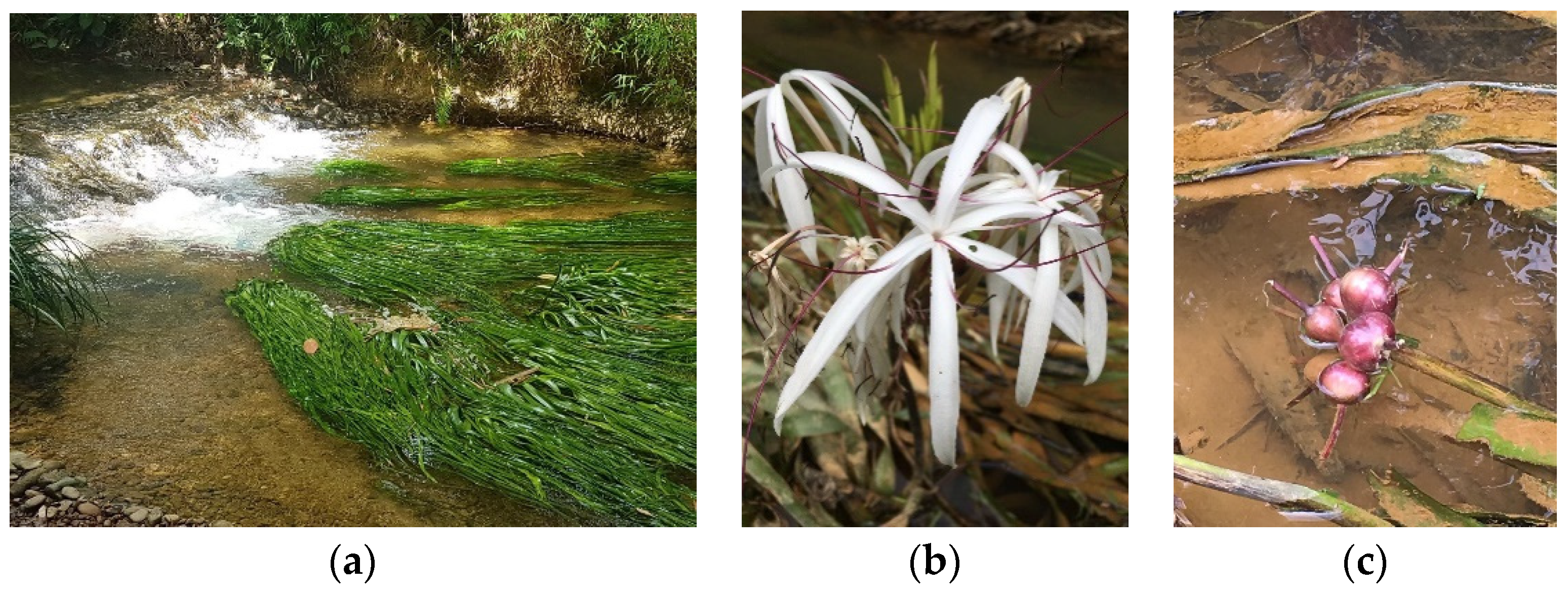
Table 1.
The attributes and attribute levels of WO habitats used in the CE survey.
| Attributes | Attributes Levels |
|---|---|
| Biodiversity | Low: the wetland has a low abundance and variety of water onions, fish, insects, animals, and other aquatic species. Medium: the abundance and variety of water onions, fish, insects, animals, and other aquatic species has increased by 25%. High: the abundance and variety of water onions, fish, insects, animals, and other aquatic species has increased by 50%. |
| Water quality | Low: low water quality; smell and algae noticeable. Medium: slightly murky water; some algae noticeable; no smell. High: water quality is very good (clear and clean); no smell. |
| Upstream condition | Low: there is a scarcity of upstream and bank vegetation, and erosion happens frequently. Medium: there is a moderate amount of upstream and bank vegetation, and a moderate chance of erosion. High: there is a lot of upstream and bank vegetation, and no danger of significant erosion. |
| Recreational opportunity | Low: visual amenity only. Medium: Secondary contact recreation possible (fishing/rafting/boating). High: All type of recreation possible, tourism infrastructures. |
| Contribution | Annual contribution. In cash: An annual donation of THB 50, 100, 200, 400, or in volunteer labor: 2, 4, 6, 12 days. |
Source: Adapted from Doherty et al. [81].
Table 2.
Example of a choice set for the CE task in monetary terms.
| Any of the following alternatives demonstrates increased benefits as a result of the WO conservation plan: Plan A and Plan B are also viable options. Which of the two options do you prefer? If you choose either option, you will incur a monetary donation. The “Neither A nor B” alternative, on the other hand, would not entail payment, but the state of ecosystem resources would not be changed. | |||
| Benefits | Plan A | Plan B | Neither A nor B: I prefer the NO conservation plan. |
| Biodiversity (abundance and variety of water onions, fish, insect, animals, and other aquatic species) |  Medium (25% increase) |  High (50% increase) | |
| Water quality | Medium Slightly murky water, some algae noticeable, no smell | High Clearwater No smell | |
| Upstream condition |  Medium abundant, moderate chance of erosion | Good High abundant No danger of significant erosion | |
| Recreational opportunity |  Low Visual amenity only |  Medium Secondary contact recreation (fishing/rafting/boating) possible | |
| Cash donation | THB 100 | THB 200 | |
| I would prefer: | ☐ | ☐ | ☐ |
Table 3.
Example of a choice set for the CE task in volunteer labor terms.
| Any of the following alternatives demonstrates increased benefits as a result of the WO conservation plan: Plan A and Plan B are also viable options. Which of the two options do you prefer? If you choose either plan, you would be expected to volunteer labor for a different number of days. The “Neither A nor B” alternative, on the other hand, would not require any labor, but the state of ecosystem resources would not be enhanced. | |||
| Benefits | Plan A | Plan B | Neither A nor B: I prefer the NO conservation plan. |
| Biodiversity (abundance and variety of water onions, fish, insect, animals, and other aquatic species) |  Low |  Medium (25% increase) | |
| Water quality | Low Low water quality, algae and smell noticeable | Medium Slightly murky water, some algae noticeable, no smell | |
| Upstream condition |  Medium abundant Moderate risk of erosion |  High abundant No danger of significant erosion | |
| Recreational opportunity |  Low Visual amenity only |  Medium Secondary contact recreation(fishing/rafting/boating) possible | |
| Volunteer labor | 6 days/year | 12 days/year | |
| I would prefer: | ☐ | ☐ | ☐ |
Table 4.
Socioeconomic characteristics of the respondents.
| Money Treatment | Labor Treatment | |
|---|---|---|
| Gender | ||
| Male | 57% | 61% |
| Female | 43% | 39% |
| Marital status | ||
| Single | 27% | 19% |
| Married | 72% | 81% |
| Age | ||
| 18–34 | 16% | 13% |
| 35–49 | 44% | 48% |
| 50–64 | 33% | 34% |
| >64 | 7% | 5% |
| Mean age in years | 46.2 | 46.1 |
| Education | ||
| <High school | 39% | 40% |
| High school | 36% | 42% |
| Bachelor’s degree | 22% | 15% |
| >Bachelor’s degree | 3% | 3% |
| Profession | ||
| Civil servants | 33% | 34% |
| Self-employed | 15% | 5% |
| Farmers | 36% | 47% |
| Employees | 12% | 10% |
| Others | 5% | 4% |
| Monthly income (THB) | ||
| <10,000 | 38% | 39% |
| 10,000–20,000 | 44% | 43% |
| 20,001–30,000 | 13% | 11% |
| >30,000 | 6% | 6% |
| Mean monthly income in THB | 13,232 | 12,632 |
| Family size (individuals) | ||
| <3 | 18% | 17% |
| 3–5 | 69% | 69% |
| >5 | 13% | 14% |
| Mean family size | 3.8 | 3.9 |
| House location | ||
| Kapoe district of Ranong | 43% | 70% |
| Suksamran district of Ranong | 19% | 30% |
| Khura Buri district of Phangnga | 30% | - |
Table 5.
Respondents’ perception, experiences, and participation regarding WO.
| Money Treatment | Labor Treatment | |
|---|---|---|
| Perceived benefits of WO | 87% | 92% |
| Perceived threats | ||
| River dredging | 57% | 63% |
| Over-exploitation | 17% | 21% |
| Land conversion in upper catchment river | 17% | 7% |
| Flooding | 7% | 7% |
| Water contamination and pollution | 2% | 2% |
| Member of an environmental conservation group | 49% | 53% |
| Participated in WO conservation | 67% | 78% |
| Voluntary in WO conservation is needed | 89% | 90% |
| Sample size, N | 267 | 166 |
Table 6.
The CL coefficient estimates for the WO case’s money treatment using two models: no socioeconomic factors (Model 1a) and socioeconomic variables (Model 1b).
Table 6.
The CL coefficient estimates for the WO case’s money treatment using two models: no socioeconomic factors (Model 1a) and socioeconomic variables (Model 1b).
| Model 1a | Model 1b | |||||
|---|---|---|---|---|---|---|
| Variable | Coefficient | T Statistic | p Value | Coefficient | T Statistic | p Value |
| Status quo | −2.9251 *** | −5.503 | 0.0000 | 1.8440 | 0.951 | 0.3417 |
| Money Cost/Payment | −0.0011 *** | −2.956 | 0.0031 | −0.0011 *** | −2.945 | 0.0032 |
| Biodiversity: high | 0.4530 *** | 6.863 | 0.0000 | 0.4518 *** | 6.845 | 0.0000 |
| Biodiversity: medium | 0.1436 ** | 2.232 | 0.0256 | 0.1440 ** | 2.238 | 0.0252 |
| Water quality: high | 0.2485 *** | 3.850 | 0.0001 | 0.2486 *** | 3.852 | 0.0001 |
| Water quality: medium | 0.0810 | 1.247 | 0.2126 | 0.0818 | 1.258 | 0.2085 |
| Upstream condition: high | 0.7872 *** | 11.617 | 0.0000 | 0.7879 *** | 11.620 | 0.0000 |
| Upstream condition: medium | 0.0804 | 1.2978 | 0.1942 | 0.0794 | 1.283 | 0.1996 |
| Recreation: high | 0.0896 | 1.3760 | 0.1689 | 0.0891 | 1.368 | 0.1712 |
| Recreation: medium | 0.0355 | 0.5680 | 0.5703 | 0.0870 | 0.573 | 0.5667 |
| Age | 0.0786 * | 1.828 | 0.0675 | |||
| Income | 0.0001 | 1.336 | 0.1816 | |||
| Log-likelihood | −522.01 | −519.04 | ||||
| No. of respondents | 242 | 242 | ||||
| No. of observation | 968 | 968 | ||||
*** 1% significance level, ** 5%significance level, * 10% significance level.
Table 7.
The CL coefficient estimates for the WO case’s labor treatment using two models: no socioeconomic factors (Model 2a) and socioeconomic variables (Model 2b).
Table 7.
The CL coefficient estimates for the WO case’s labor treatment using two models: no socioeconomic factors (Model 2a) and socioeconomic variables (Model 2b).
| Model 2a | Model 2b | |||||
|---|---|---|---|---|---|---|
| Variable | Coefficient | T Statistic | p Value | Coefficient | T Statistic | p Value |
| Status quo | −2.4563 *** | −4.504 | 0.0000 | −3.4247 | −1.506 | 0.1320 |
| Labor Cost/Payment | −0.0421 *** | −2.666 | 0.0077 | −0.0420 *** | −2.661 | 0.0078 |
| Biodiversity: high | 0.4320 *** | 4.890 | 0.0000 | 0.4341 *** | 4.904 | 0.0000 |
| Biodiversity: medium | 0.0204 | 0.249 | 0.8036 | 0.0204 | 0.248 | 0.8039 |
| Water quality: high | 0.4158 *** | 4.647 | 0.0000 | 0.4191 *** | 4.671 | 0.0000 |
| Water quality: medium | 0.1616 | 0.197 | 0.8441 | 0.0154 | 0.187 | 0.8518 |
| Upstream condition: high | 0.6345 *** | 7.822 | 0.0000 | 0.6346 *** | 7.816 | 0.0000 |
| Upstream condition: medium | 0.4118 *** | 4.944 | 0.0000 | 0.4134 *** | 4.957 | 0.0000 |
| Recreation: high | 0.0844 | 1.376 | 0.1689 | 0.0835 | 1.001 | 0.3167 |
| Recreation: medium | −0.0960 | −1.179 | 0.2383 | −0.0972 | −1.193 | 0.2330 |
| Age | −0.0031 | −0.060 | 0.9525 | |||
| Income | −0.4551 * | −1.924 | 0.0544 | |||
| Log-likelihood | −320.25 | −318.11 | ||||
| No. of respondents | 148 | 148 | ||||
| No. of observation | 592 | 592 | ||||
*** 1% significance level, * 10% significance level.
Table 8.
MWTP and MWTV for each attribute improvement, and the total WTP and WTV of improved WO ecosystem services (per person per year).
Table 8.
MWTP and MWTV for each attribute improvement, and the total WTP and WTV of improved WO ecosystem services (per person per year).
| Attribute | Improved Level | MWTP (THB/Person/Year) | Improved Level | MWTV (Days/Person/Year) | ||||
|---|---|---|---|---|---|---|---|---|
| Low | Medium | High | Low | Medium | High | |||
| Biodiversity | −564 | 136 | 428 | 992 | −10.2 | − | 10.2 | 20.4 |
| Water quality | −235 | − | 235 | 470 | −9.9 | − | 9.9 | 19.8 |
| Upstream condition | −744 | − | 744 | 1488 | −24.9 | 9.8 | 15.1 | 40 |
| Recreation | − | − | − | − | ||||
| Total | 2950 | 80.2 | ||||||
THB 1 = USD 0.03 (1 September 2019).
Publisher’s Note: MDPI stays neutral with regard to jurisdictional claims in published maps and institutional affiliations. |
© 2022 by the authors. Licensee MDPI, Basel, Switzerland. This article is an open access article distributed under the terms and conditions of the Creative Commons Attribution (CC BY) license (https://creativecommons.org/licenses/by/4.0/).
Share and Cite
MDPI and ACS Style
Petcharat, A.; Jo, J.-H.; Lee, Y. Comparing Local Residents’ Willingness to Pay (WTP) and Willingness to Volunteer (WTV) for Water Onion (Crinum thaianum) Habitat Conservation. Forests 2022, 13, 706. https://doi.org/10.3390/f13050706
AMA Style
Petcharat A, Jo J-H, Lee Y. Comparing Local Residents’ Willingness to Pay (WTP) and Willingness to Volunteer (WTV) for Water Onion (Crinum thaianum) Habitat Conservation. Forests. 2022; 13(5):706. https://doi.org/10.3390/f13050706
Chicago/Turabian StylePetcharat, Areeyapat, Jang-Hwan Jo, and Yohan Lee. 2022. "Comparing Local Residents’ Willingness to Pay (WTP) and Willingness to Volunteer (WTV) for Water Onion (Crinum thaianum) Habitat Conservation" Forests 13, no. 5: 706. https://doi.org/10.3390/f13050706
Note that from the first issue of 2016, this journal uses article numbers instead of page numbers. See further details here.